I ran the Richmond Marathon in 2019 and I loved a lot of things about it. It was a challenging race for me. The course was fun but did feature some long inclines. The threat of rain did not materialize, but we did have 15-20 mile per hour wind with gusts up to 30. I finished with a good time, but I don't think any metrics could capture what I accomplished. I started wondering about the metrics that are available from the Richmond Marathon, and I decided to take a look at most improved.
I compiled a spreadsheet for the runners of the race in 2018 and 2019. I had to get through some data grooming before I could really compare anything. I wanted to look at runners who ran the race both years. The best approach I could take from the data available was to look for runners with the same name,and filter out results when age between the two races didn't make sense. Unfortunately, this strategy means if your name didn't appear the same, or you changed your name between races, I can't understand you are the same runner. If this applies to you, please let me know.
I combined the results from both years as data frames and joined them based on the name, to create a set of people who appeared in results from both years, and found 728. I filtered out people who had the same name but had a younger age in 2019 than in 2018, and I filtered out people with the same name but aged more than 2 years between the races. That leaves 709 runners. It came in handy that I learned in my last project you can ask Python to use timedelta64 for race time, and that will make math easier. I added columns to show the difference in time, and then sorted based on that value.
You might notice that this marathon, like most races, captures two times for each runner. In the results you'll see 'net' time and 'gun' time. Gun time refers to the time between when they officially started the race and the time you cross the finish line. Net time (sometimes called chip time) is the difference between when you cross the start line and the finish line. In larger races it can take a substantial amount of time to get to the start line. Elite runners are often put at the front of the race so that they can get a lower gun time, often used for prizes. Since we have the technology to know your net used the net time rather than the gun time, I think it's pretty silly to consider gun time. I used net time for this analysis.
Kevaughn Smith of Newark, New Jersey improved his time more than any other runner. In 2018 he ran a net time of 6:03:06, and In 2019 his time was 4:15:08. Incredible improvement! 4:15 is also an impressive time considering the wind gusts in 2019. Most improved female was Victoria Hebert of Lynchburg, Virginia. Victoria ran a 6:34:33 in 2018 and a 5:17:21 in 2019. Way to go Victoria!
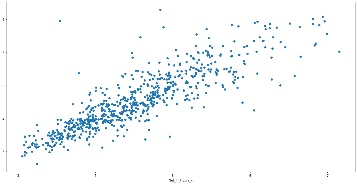
I also plotted out the results, for each runner showing the 2018 time on the horizontal axis and 2019 time on the vertical axis. You can see the data is about what we expect, most people ran about the same time each year. There is apparently a problem in Python plotting values that are timedelta, and there is a note on GitHub about it. I created an additional column to convert the times to hours. For instance, 3:30:00 would appear as 3.5. I added this value so that Python would be able to put the number on the graph. You can see that most runners had similar times from 2018-2019 so there is a nice trend to the distribution.

One of the things that I love about looking at data at scale, like in this project, and finding impressive performances like these. When you finish a race like Richmond, such a big experience with many ups and downs, it's tempting to look at the time on your watch and want the time on it to represent all that has happened. I'm sure that Kevaughn and Victoria realized they made huge improvements over their previous times, but unless you digest all the data, they wouldn't know they improved the most of all of the runners. If you know Kevaughn or Victoria, please pass on the news!
You can access my Jupyter Notebook on GitHub, or in Binder. If you are new to Jupyter Notebook I posted some easy to follow steps so that you can see under the hood or download a copy of all of the results.